Why we use multifactor models
Right, so this blog will be written in English, even if our customers in Praxis Capital are all Norwegian (actually we do have one Swede, but he has lived here so long I’m not sure he counts as Swedish anymore:)). I like to discuss ideas with people outside of Norway too, so English it is.
—
On to the topic of this post: Praxis runs a portfolio of systematic equity strategies, each with a different focus area. One is primarily momentum focused, another is primarily quality focused etc. However, none of the sub-strategies use only one factor, they are all multi-factor models. Why do we construct all our strategies that way? We believe that:
Single factor models are more vulnerable to periodic underperformance, so using more factors increases model robustness
First of all, because it helps us reduce unwanted negative factor loadings in the models. A momentum strategy will tend to do better with a volatility measurement added on for example, while a quality strategy might benefit from adding value metrics.
In the case of the momentum strategy, the reason is fairly intuitive: it reduces the risk of momentum crashes and makes it easier to stick with the strategy in bad times (which you can be sure will come from time to time).
The value metrics might help an investor avoid the good companies that are already priced to, or beyond, perfection. History is littered with examples of good companies that became so expensive that the expected returns became unacceptably low and left investors wandering the desert for years if they stuck around.
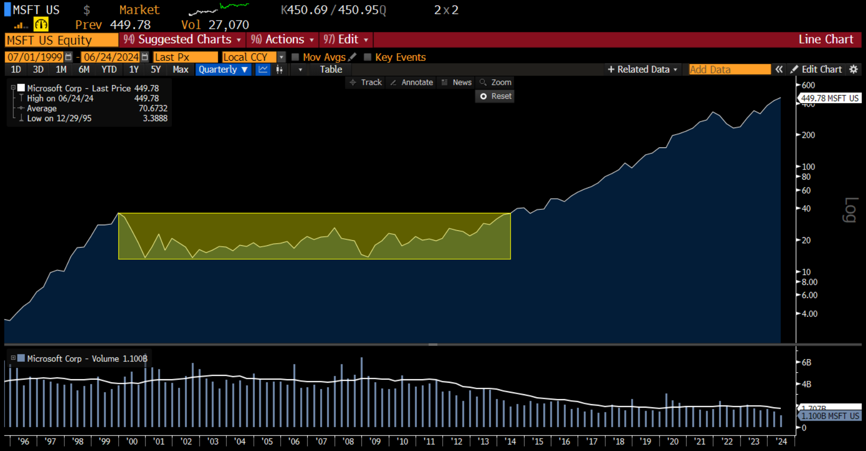
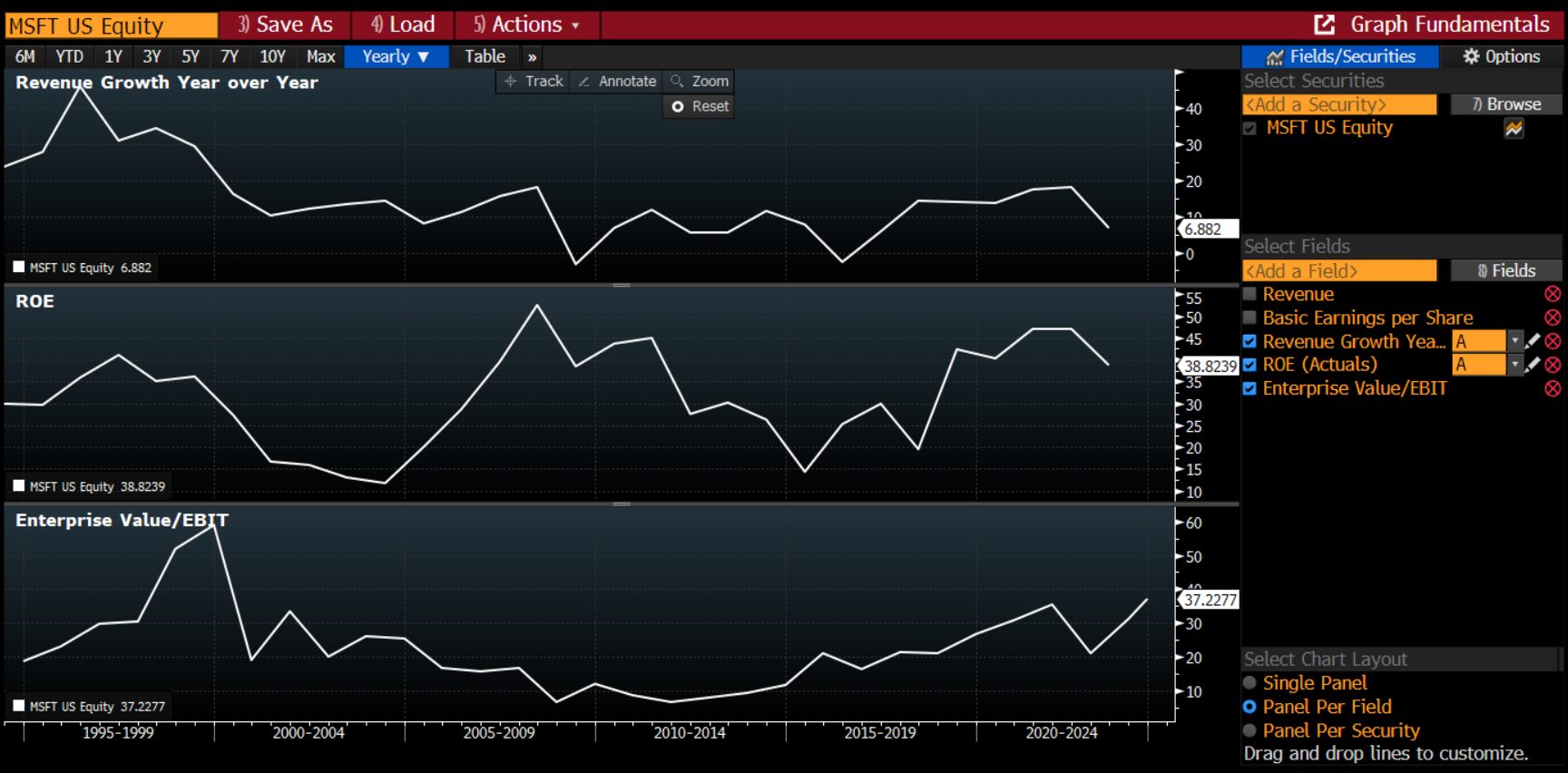
For example, Microsoft was obviously a very good company in 1999. At that point in time, the trailing 12m revenue growth was > 30%, and the ROE > 40%. There was a problem, however. The valuation reflected this quality and then some. The trailing 12m EV/EBIT multiple was 59x! That EV/EBIT multiple would contract all the way to < 10x by year end 2012. (Recently, the EV/EBIT multiple has expanded again to almost 40x, and MSFT shares are up >2000% since early 2012). Clearly, valuation matters a great deal over long time periods (but very little in the short term).
Despite the quality of the company, an investor who bought MSFT in september 1999 would have to wait 14.5 years for a new all time high, even when including dividends! Obviously, this is the kind of situation we’d like to avoid.
Bloomberg data
Bloomberg data
2. Over time, multifactor models also tend to produce higher returns than single-factor models
First, we’ll define a set of variables that we think are correlated with higher future returns. We’ll use relatively simple examples here. Higher values of the variable are believed to be a positive thing. We are only interested in potential long exposure.
Return on equity (ROE), 5 year average. A quality metric.
Idiosyncratic momentum, 12m-1m excess returns vs benchmark / volatility.
Equity / net debt. A robustness metric.
Book value to price. A classic value metric.
5-year sales growth.
How do these predictors relate to future returns, and over what timeframes are they most predictive?
Let’s run a little experiment to find out. We’ll use a universe of the 200 largest stocks in the Nordic region by market capitalization, measured on the final trading day of 2010. Any stock with missing values for any of our chosen predictive metrics is disregarded. The universe includes delisted stocks. After cleaning the data set for stocks with missing data, we are left with 158 stocks.
We’ll divide the stocks in the universe into quantiles based on their ranks on the various metrics so that the highest ranked stocks (1 is the best, 158 is the worst) are put in quantile 0 and the lowest ranked stocks are put in quantile 4. For the sake of brevity I won’t post detailed results for all predictors, but below I show how the tables look for the two first predictors listed above, along with a brief comment.

5-year average ROE
The stocks with the highest 5 year avg ROE (quintile 0) have the highest total returns over the next 3 months, and also do very well over the 1,2 and 3 year measurement periods. Over 5 a years the relatonship is less clear, and over 10 years, the lowest quantile ROE stocks outperform markedly. It should be noted though that the bottom quantile return over 10 years is driven by a few positive outliers - the median stock in the bottom quantile does poorly.

Idiosyncratic momentum
For IMOM, the highest ranked stocks outperform all other quintiles over every timeframe except 10 over years, where it comes in second, narrowly behind quantile 2. The two bottom quintiles perform the worst across all timeframes. Top quantile IMOM names perform better than top quantile ROE names across all timeframes.
Summarizing the other predictors performance per quantile:
Equity to net debt:
High debt may be risky, but it appears not to be a compensated risk. Top quantile equity to net debt tends to outperform the bottom quintile, with the exception of the 10 year period. But again, looking at this in more detail (plot not shown) reveals that this 10 year result is driven by a handful of positive outliers in the bottom quantile - most high debt stocks do badly over 10 years as well.
Book value to price:
This predictor has no monotonic relationship with subsequent returns in this sample. The results are kind of murky. What is clear in this data set is that top ranked B/P stocks do poorly in the short to medium term and better over the long term, with strong absolute returns on par with IMOM over 10 years.
5 year sales growth:
High sales growth predicts higher returns in the short term (3 months), after which the relationship becomes unclear. Over 10 years, the highest growth companies do better than the lowest growth companies, but not better than the middle quantiles.
What happens if we combine the predictors into a single ranking?
After combining the rankings on the 5 individual metrics, we run the same experiment again. How do the top quantile (0) stocks perform versus the bottom quantile (5)? Is the relationship clearer than for individual predictors?
First, let’s look at some scatter plots of combined ranks and returns. Higher ranked stocks clearly tend to outperform lower ranked stocks. Note that this is a combined ranking, so that the top ranked stock is not ranked 1 (but rather assigned the average rank across predictors).
The outperformance is evident whether we look at the relationship over the shorter term or the longer term:

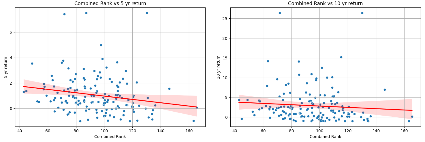
Higher returns for the combined rank model? Yes.
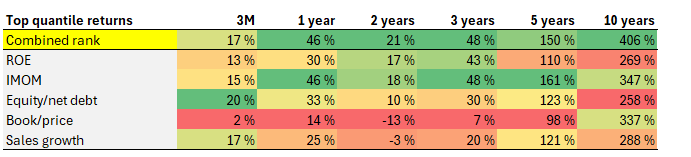
Top quantile combined rank stocks outperform all individual predictors over almost every single timeframe. The best individual predictor is idiosyncratic momentum.
How strong is the relationship between combined rank and returns?
Spearman’s rank correlation measures the strength and direction of association between two ranked variables. The Spearman Rank Correlation can take a value from +1 to -1 where:
A value of +1 means a perfect association of rank
A value of 0 means that there is no association between ranks
A value of -1 means a perfect negative association of rank
These results show that there is a negative correlation between the combined rank and returns across all periods: lower combined ranks (better rankings) are associated with higher subsequent returns and higher combined rank scores are associated with lower subsequent returns (if you were wondering why the coefficients were negative in the table below).

Interpreting the Spearman rank correlation coefficients across timeframes
First of all, it seems the relationship is strongest over the shortest timeframe. Generally, better rankings appear to be associated with higher returns. As would be expected, the relationship is relatively weak (but in my opinion exploitable).

Returns across quantiles
The top ranked stocks tend to outperform lower ranked stocks across all timeframes.

Top ranked quantile versus bottom ranked quantile
There is a meaningful difference in returns between top and bottom ranked stocks across all timeframes. The difference becomes huge over 5 and 10 years.
Conclusions / take-aways:
If you want to win a basketball game, you don’t want a team where one person is only great at 3-point shooting, the other only great in dribbling, and the other only great at passing the ball. You want a team with players who stand out at shooting but are also good at dribbling and passing the ball. An individual sleeves approach will invest in stocks that are high value and very low momentum or other factor dimensions.
Liqian Ren, Wisdom Tree
The relationship between rank and return is positive for some individual predictors. However, it tends to break down over the longer timeframes. (The exception is book to price, which works best over longer timeframes but is heavily driven by a few positive outliers. Which means most cheap stocks are cheap for a reason and will not do well even if you’re patient. That’s my interpretation anyway).
The relationship between rank and return appears much more stable and consistent when we use multiple predictors (factors).
The difference between top combined-ranked and bottom combined-ranked stocks becomes very large over longer timeframes.
As a result, we prefer to build models based on multiple predictors/factors - they seem more robust and less risky.
While you can achieve some of the same effect of multifactor models by combining single factor models together (so-called factor sleeves: having a clean sub-portfolio of value stocks along side a clean sub-portfolio of momentum stocks for example), we believe combining multifactor models with different focus areas (a tilt toward a specific factor) is a better way to go.
This allows us to sidestep stocks that are particularly weak in certain aspects (e.g. an extremely cheap stock with terrible return momentum, or a high-momentum score stock with astronomical valuation). We also think it helps reduce portfolio turnover.
PS: Not everyone agrees with us on this. A good further discussion of this topic and the pros and cons of sleeves versus integration can be found here, if you’re interested. Thanks for reading!